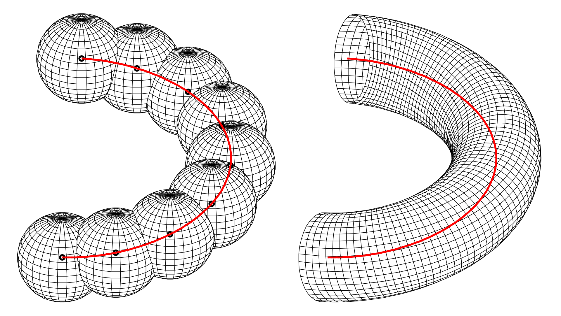
Channel as a sweep of sphere
A channel is a surface formed as the envelope of a family of spheres, each with its center on a space curve called the directrix. We’ll generalize this definition to ellipsoids for our specific case. Channel surfaces in topology are formed by sweeping a sphere along a directrix. The directrix determines whether the channel surface is open or closed.
- Right circular cylinder: When the directrix is a straight line and the radii are constant.
- Torus: When the directrix is a circle and the radii are constant.
- Right circular cone: When the directrix is a straight line and the radii decrease to zero.
We aim to plot a channel in MATLAB using two directrices as focal points of rotational ellipsoids. We assume that the two axes other than the focal axis are equal (\(b = c\)), which we will refer to as the minor axis or axes. We are provided with a list of discrete position coordinates for the two directrices and the corresponding lengths of either the semi-major or the semi-minor axis.
\[F_{1} = \left\{ \left( p_{i} , q_{i} , r_{i} \right) \right\}\] \[F_{2} = \left\{ \left( u_{i} , v_{i} , w_{i} \right) \right\}\] \[A = \left\{ a_{i} \right\} ,or, B = \left\{ b_{i} \right\}\]
Data is stored in a MATLAB readable text file in seven rows for p, q, r, u, v, w, a or b.
To plot a surface in MATLAB, we use surf(x,y,z) where \(x, y, z\) are matrices of second order and dimensions \(m \times n\).
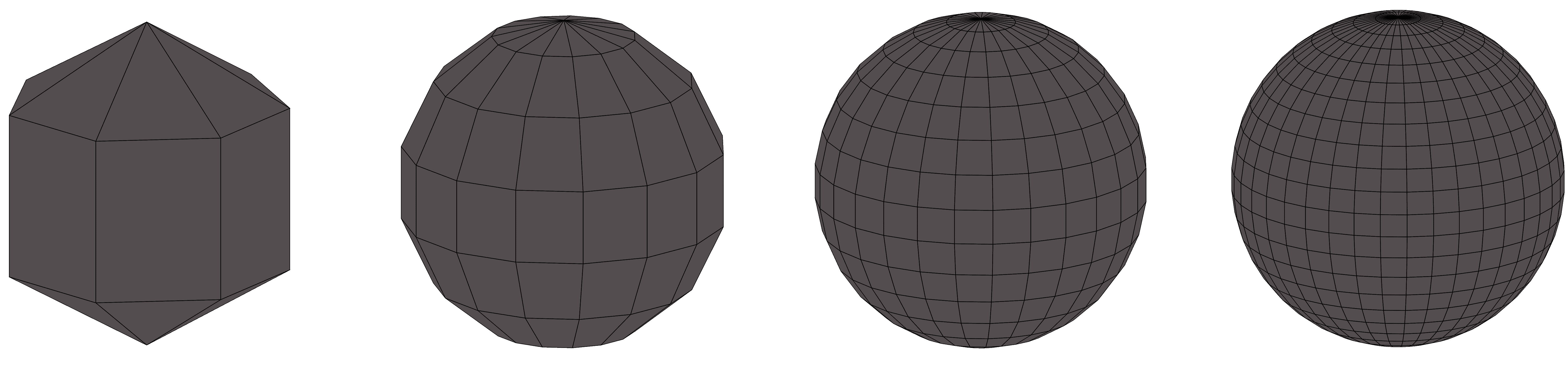
Sphere as mesh of various densities
A “sheet” of points, used by MATLAB to create a mesh of a surface for plotting, consists of columns and rows that form intersecting curves which create a net that MATLAB fills.
If the data is stored in MATLAB-readable format in a text file, such as curves.txt, we can use the load() function to extract all the data into a variable and then distribute it among various variables.
impdata = load("curves.txt", "~ascii");
p      = impdata(1,:);
q      = impdata(2,:);
r      = impdata(3,:);
u      = impdata(4,:);
v      = impdata(5,:);
w      = impdata(6,:);
minor  = impdata(7,:);
clear impdata;
To simplify the mathematics of a channel, we will make an analogy to one of its special cases, a right cylindrical surface.
A right cylindrical surface is a channel formed by a series of spheres, with their directrix being a line. Alternatively, a solid cylinder can be thought of as the result of integrating circular discs oriented perpendicular to the directrix. A cylindrical surface, on the other hand, is the result of integrating circles or the perimeters of the discs.
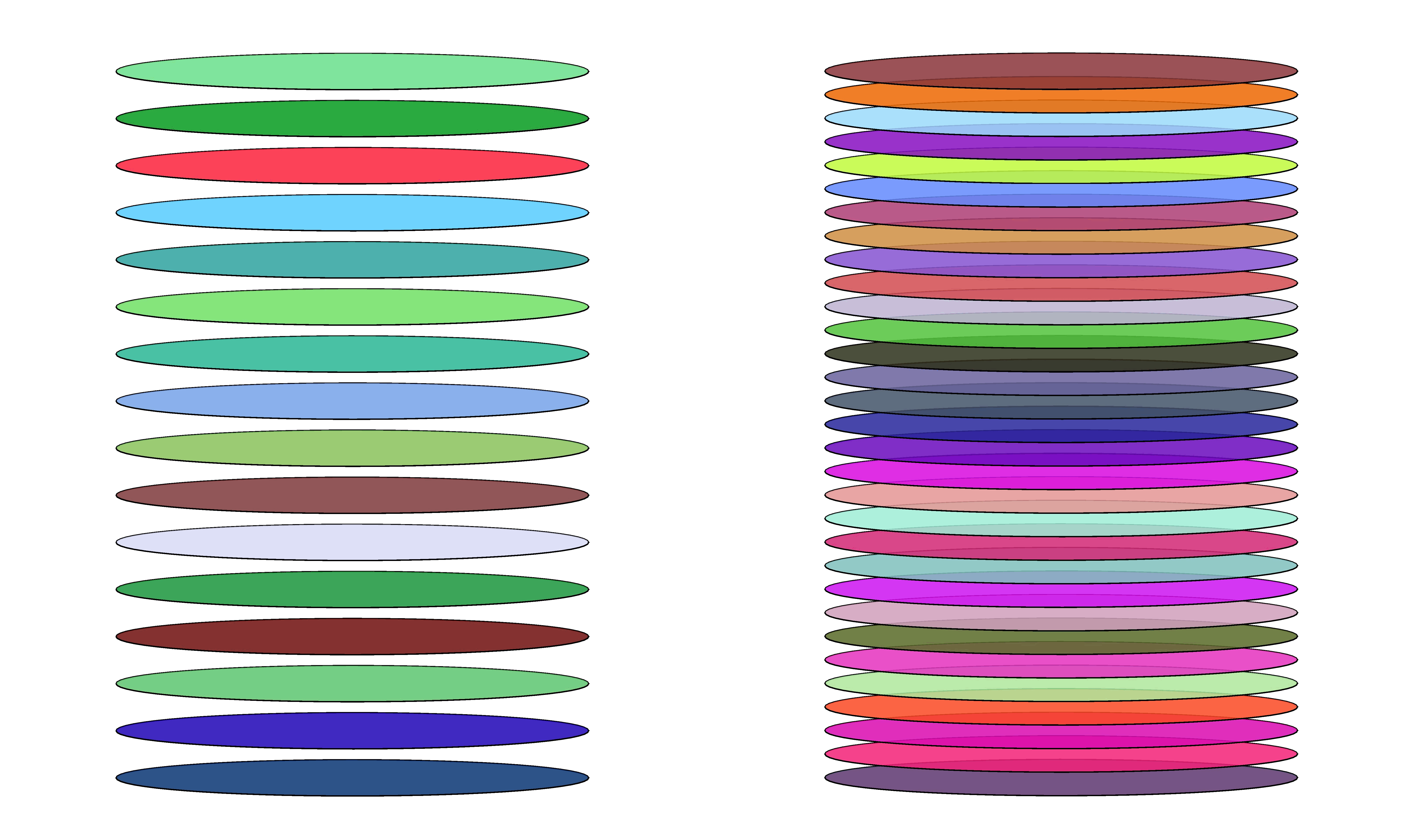
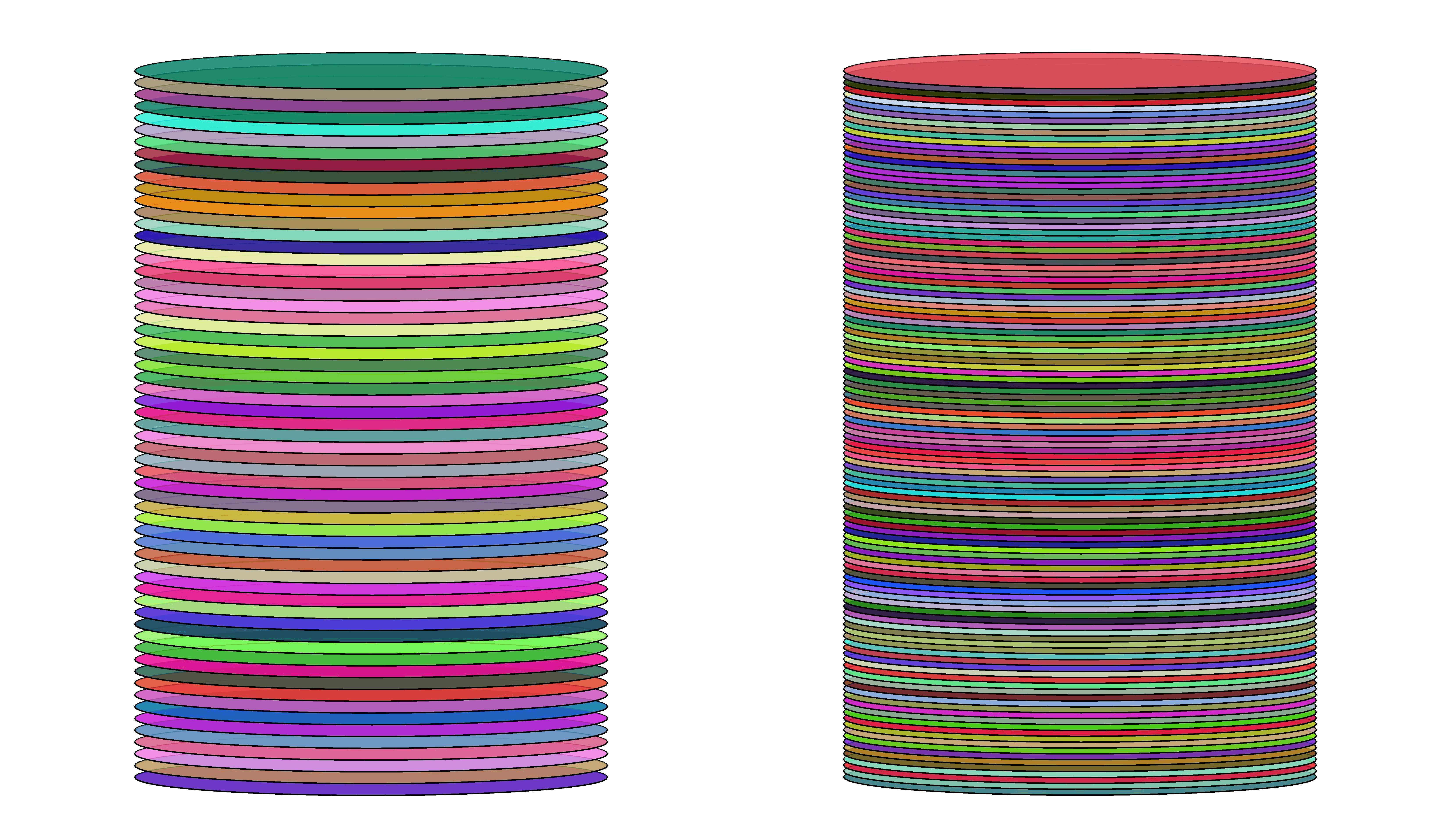
Cylinder as Integration of Circular Sheets
We can visualize a channel as a cylinder with varying cross-sectional radii. This allows us to calculate the position of points on elliptical cross-sections to create a mesh of the channel.
After calculating the Directrix,
\[D = \frac{F_{1} + F_{2}}{2}\]
We are provided with a minor axis length as well, so we will also determine focal length & Directrix coordinates, and calculate major axis length.
focal = sqrt( (p-u).^2 + (q-v).^2 + (r-w).^2) / 2;
major = sqrt(focal.^2 + minor.^2);

x = (p+u)/2;
y = (q+v)/2;
z = (r+w)/2;
By default, MATLAB attempts to perform matrix operations on arrays; that is, using multiplication and squaring results in matrix multiplication. Therefore, operations are modified with a period (.) to make them element-wise. For example, .^2 squares each element individually, and sqrt() applies element-wise.
We have one more necessary parameter to determine: the tangents of the directrix. Since we are dealing with a set of discrete points, there are a few techniques that we can use for calculating tangents.
\[\vec{R} = \left(\, x(t)\, ,\, y(t) \, ,\, z(t)\, \right)\]
A one dimensional object, like a line or a curve, suspended in a three dimensional space can be represented as each coordinate being a function of some independent parameter t.
Slope is given by: \[\vec{M} = \left(\, \frac{\partial x}{\partial t} \, ,\, \frac{\partial y}{\partial t}\, ,\, \frac{\partial z}{\partial t}\, \right)\]
If \(t := x\), then:
\[\vec{R} = \left( \,x\, ,\, y(x) \, ,\, z(x) \,\right)\] \[\vec{M} = \left( \,1 \, ,\, \frac{\partial y}{\partial x} \, ,\, \frac{\partial z}{\partial x}\, \right)\]
Global polynomial fitting involves approximating a dataset using a single polynomial equation of degree k that best represents the data. Once fitted, the polynomial can be differentiated to compute derivatives (e.g., slopes) at any given data point.
Calculating the slope of a curve can be quite tedious to code. First, we need to determine the coefficients of the fitted polynomial and then use these coefficients to calculate the derivative of the polynomial at each point. MATLAB’s built-in functions polyfit(x,y,k), polyder(func), and polyval(func,val) simplify this process.
% Degree of the polynomial fit
polynomial_order = 3;  % Choose based on the complexity of the data

% Number of points in the dataset
count = size(x, 2);

% Fit polynomials globally for y and z
p_y = polyfit(x, y, polynomial_order);  % Polynomial coefficients for y
p_z = polyfit(x, z, polynomial_order);  % Polynomial coefficients for z

% Compute the derivative coefficients
dp_y = polyder(p_y);  % Derivative coefficients for y
dp_z = polyder(p_z);  % Derivative coefficients for z

% Initialize arrays to store tangents (derivatives) at each point
tangent_y = zeros(1, count);
tangent_z = zeros(1, count);

% Evaluate the derivative polynomials at each point in x
for n = 1:count
tangent_y(n) = polyval(dp_y, x(n));  % Derivative of y at x(n)
tangent_z(n) = polyval(dp_z, x(n));  % Derivative of z at x(n)
end
Operational Complexity:
- Polynomial Fitting (
polyfit): \( O(n \cdot k + k^3) \) where \( n \) is the number of points and \( k \) is the degree. - Derivative Computation (
polyder): \( O(k) \) for each polynomial. - Polynomial Evaluation (
polyval): \( O(n \cdot k) \).
Total Complexity: \(O(n \cdot k + k^3)\)
Key Observations:
- For large \( n \), the term \( O(n \cdot k) \) dominates.
- For large \( k \), the cubic cost \( O(k^3) \) dominates.
- The code is efficient for small \( k \) but becomes computationally expensive for high-degree polynomials.
Limitations: Overestimation or underestimation may occur if the proper degree is not used.
Spline interpolation is a piecewise polynomial method used to approximate a dataset by constructing smooth polynomials between consecutive points. It avoids overfitting and instabilities seen in global polynomial fitting.
window_size = 5;    % Number of points in the fitting window
max_order   = 3;    % Maximum degree of the polynomial fit
count       = size(x, 2); % Total number of points

tangent_y = zeros(1, count);
tangent_z = zeros(1, count);

for n = 1:count
% Determine the indices for the fitting window
half_window = floor(window_size / 2);
start_idx = max(1, n - half_window);
end_idx = min(count, n + half_window);

x_window = x(start_idx:end_idx);
y_window = y(start_idx:end_idx);
z_window = z(start_idx:end_idx);

% Determine the polynomial order based on the window size
current_order = min(max_order, length(x_window) - 1);

p_y = polyfit(x_window, y_window, current_order);
p_z = polyfit(x_window, z_window, current_order);

dp_y = polyder(p_y);
dp_z = polyder(p_z);

tangent_y(n) = polyval(dp_y, x(n));
tangent_z(n) = polyval(dp_z, x(n));
end
Operational Complexity:
- Polynomial Fitting (
polyfit): \( O(m \cdot k^2 + k^3) \) where \( m \) is the window size and \( k \) is the degree. - Derivative Computation (
polyder): \( O(k) \). - Polynomial Evaluation (
polyval): \( O(k) \).
Total Complexity per iteration: \(O(m \cdot k^2 + k^3)\)
Limitations: MATLAB’s polyfit may error if consecutive data points are too close (e.g., differences less than \(0.01\)).
Line connecting two points is the slope at some point between them
This method is based on Lagrange's mean value theorem which states that in any interval \(\lbrack a,b\rbrack\), there is some \(c\) for which:
\[f^{'}(c) = \frac{f(b) - f(a)}{b - a}\]
We assume that \(c\) is close enough to our point that we can approximate its tangent as being equal to our point.
count = size(x, 2);

tangent_y = zeros(1, count);
tangent_z = zeros(1, count);

tangent_y(1) = (y(2) - y(1)) / (x(2) - x(1));
tangent_z(1) = (z(2) - z(1)) / (x(2) - x(1));

tangent_y(end) = (y(end) - y(end-1)) / (x(end) - x(end-1));
tangent_z(end) = (z(end) - z(end-1)) / (x(end) - x(end-1));

for n = 2:count-1
tangent_y(n) = (y(n+1) - y(n-1)) / (x(n+1) - x(n-1));
tangent_z(n) = (z(n+1) - z(n-1)) / (x(n+1) - x(n-1));
end
Spline interpolation excels where finite difference fails, and vice versa.
| Global Fitting | Spline Fitting | Finite Difference | |
|---|---|---|---|
| Process | Fit a single \( k \)-th degree polynomial to all data points, then differentiate. | Fit \( n \) piecewise \( k \)-th degree polynomials, then differentiate each segment. | Use finite differences between neighboring points to estimate derivatives. |
| Strengths | Smooth, continuous data; small to medium datasets. | Handles sharp transitions, non-uniform spacing, or local trends. | Efficient for smooth, evenly spaced data. |
| Weaknesses | Risk of overfitting or instability with high-degree polynomials. | Higher computational cost and potential errors with very dense data. | Highly sensitive to noise and unsuitable for uneven spacing. |
| Complexity | \( O(nk^2 + k^3) \) | \( O(nk^2 + nk) \) | \( O(n) \) |
Data that we use as test data is very dense and smooth. Therefore, we will use the Central Finite Difference.
Special points and parameters of an ellipse
An ellipse is a locus of points in a plane whose distances from two focal points have a constant sum. Let the focal points be \(C_{1}\) and \(C_{2}\), with \(O\) as their midpoint (the ellipse's center). For any point \(P\) on the ellipse, \(C_{1}P + C_{2}P = k\).
The line passing through the focal points is the Major Axis, and the line perpendicular to it (passing through the center) is the Minor Axis.
Let \(OA = a\) be the semi-major axis, \(OB = b\) be the semi-minor axis, and \(OC = c\) be the focal distance from the center. Useful relations include:
\(a = \frac{k}{2}\)
\(a^{2} = b^{2} + c^{2}\)
The vector equation of an ellipse is given by:
\(\vec{r} = a \cdot \cos(\theta)\ \hat{i} + b \cdot \sin(\theta)\ \hat{j} + \vec{O}\)
More generally, using any pair of mutually perpendicular unit vectors:
\(\vec{r} = a \cdot \cos(\theta)\ \hat{a} + b \cdot \sin(\theta)\ \hat{b} + \vec{O}\)
Representing a point \(x\hat{i} + y \hat{j} + z\hat{k}\) as a matrix:
\(\begin{bmatrix}r_{x} & r_{y} & r_{z}\end{bmatrix} = a\begin{bmatrix}\cos(\theta)a_{x} & \cos(\theta)a_{y} & \cos(\theta)a_{z}\end{bmatrix} + b\begin{bmatrix}\sin(\theta)b_{x} & \sin(\theta)b_{y} & \sin(\theta)b_{z}\end{bmatrix}\)
Channel Directrix is the curve that passes through the centers of all ellipses.
\(D = \frac{F_{1} + F_{2}}{2}\)
Each ellipse must satisfy:
- Major Axis must pass through the Focal Points.
- Ellipses must be perpendicular to the Directrix; that is, the normal vector of the ellipse is tangential to the directrix.
- Major and Minor Axes must be mutually perpendicular.
In practice, it is challenging to satisfy all conditions. Therefore, we choose to enforce that the Major Axis always passes through the Focal Points.
Let \(\hat{n}\) be a unit tangent vector to the Directrix. Then:
\(\hat{a} = \frac{1}{2}\frac{\begin{bmatrix} F_{x}^{2} - F_{x}^{1} & F_{y}^{2} - F_{y}^{1} & F_{z}^{2} - F_{z}^{1} \end{bmatrix}}{\sqrt{(F_{x}^{2} - F_{x}^{1})^{2} + (F_{y}^{2} - F_{y}^{1})^{2} + (F_{z}^{2} - F_{z}^{1})^{2}}}\)
\(\hat{b} = \hat{n} \times \hat{a}\)
\(\hat{a} = \hat{b} \times \hat{n}\)
Thus, the minor axis is always perpendicular to the tangent of the directrix.
To generate each elliptical cross-section, MATLAB computes the major and minor axes for each ellipse, then shifts the points by the ellipse’s center coordinates.
t      = 0:0.01:2*pi+0.1;
cyl_x  = zeros(size(t'*x));  % Container matrices for coordinates
cyl_y  = cyl_x;
cyl_z  = cyl_x;

for n = 1:size(x,2)
norm_vec  = [1 tangent_y(n) tangent_z(n)];
norm_vec  = norm_vec / norm(norm_vec);  % Unit vector
focal_vec = [(p(n)-u(n))/2 (q(n)-v(n))/2 (r(n)-w(n))/2];
minor_vec = cross(norm_vec, focal_vec);
minor_vec = minor_vec / norm(minor_vec);
major_vec = focal_vec / norm(focal_vec);
point_vec = (major(n) * (cos(t)' * major_vec) + minor(n) * (sin(t)' * minor_vec));

% Each column corresponds to one elliptical cross-section
cyl_x(:,n) = point_vec(:,1);
cyl_y(:,n) = point_vec(:,2);
cyl_z(:,n) = point_vec(:,3);
end

k       = ones(size(t));
shift_x = k' * x;
shift_y = k' * y;
shift_z = k' * z;
cyl_x   = cyl_x + shift_x;
cyl_y   = cyl_y + shift_y;
cyl_z   = cyl_z + shift_z;
All the code described above is compiled into one .m file and executed in MATLAB. The surf() function is used to plot the surface. The resultant surface object has several modifiable properties:
- EdgeAlpha (0–1): Opacity of mesh edges (set to 0 to avoid darkening).
- FaceColor: Surface color (using "interp" for gradient shading based on z-value).
- FaceLighting: Defines the light source for the surface.
- SpecularStrength (0–1): Controls surface glossiness.
- AmbientStrength (0–1): Controls ambient light intensity.
g_cyl = surf(cyl_x, cyl_y, cyl_z);
g_cyl.EdgeAlpha        = 0;
g_cyl.FaceColor        = "interp";
g_cyl.FaceAlpha        = 1;
g_cyl.FaceLighting     = "gouraud";
g_cyl.AmbientStrength  = 0.6;
g_cyl.SpecularStrength = 0.2;

axis equal;
axis auto;
xlabel("x-axis");
ylabel("y-axis");
zlabel("z-axis");
grid on;
Following code generates test data for all subsequent figures:
helix_rad     = 6;
helix_stretch = 10;
x             = 0:0.1:50;
a             = helix_rad * cos(1*x/helix_stretch - pi/4);
b             = helix_rad * sin(1*x/helix_stretch - pi/4);
rad           = (sin(pi*sin(x/8).^2) + cos(3*pi/2*sin(x/7)) + exp((x-5)/35)) + 1;
c             = -1 * helix_rad * cos(1.2*x/helix_stretch - pi/4);
d             = -1 * helix_rad * sin(1.1*x/helix_stretch - pi/4);
save("curves.txt", "x", "a", "b", "x", "c", "d", "rad", "-ascii");
Rendering of Calculated Mesh
To enhance the plot, boundaries around a few cross-sections are added by plotting only selected columns.
hold on
cross_density = 15;
g_cross = plot3(cyl_x(:, 1:1+cross_density:end), ...
            cyl_y(:, 1:1+cross_density:end), ...
            cyl_z(:, 1:1+cross_density:end), ...
            'LineWidth', 1);
Plots of Cross-sections only
plot3 plots each column as an individual curve when given a matrix.
Channel with sparsely marked cross-sections
Shadows are added by plotting the surface again with one axis scaled almost to zero and shifted to create a projection.
shadow_xy = surf(cyl_x, cyl_y, cyl_z * 0.01 - 15);
shadow_xz = surf(cyl_x, cyl_y * 0.01 + 15, cyl_z);
shadow_yz = surf(cyl_x * 0.01 - 15, cyl_y, cyl_z);

shadow_xy.EdgeAlpha = 0;
shadow_xy.FaceColor = [0, 0, 1];
shadow_xy.FaceLighting = "gouraud";
shadow_xy.FaceAlpha = 0.15;

shadow_xz.EdgeAlpha = 0;
shadow_xz.FaceColor = [0, 0, 1];
shadow_xz.FaceLighting = "gouraud";
shadow_xz.FaceAlpha = 0.15;

shadow_yz.EdgeAlpha = 0;
shadow_yz.FaceColor = [0, 0, 1];
shadow_yz.FaceLighting = "gouraud";
shadow_yz.FaceAlpha = 0.15;
Channel with cross-sections and shadows